知识补全(不定期更新)
拉普拉斯矩阵(Laplacian Matrix)
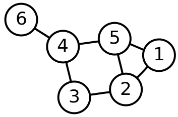
对于一张图G = ( V , E ) G=(V,E) G = ( V , E ) L L L L = D − A L=D-A L = D − A D D D A A A
其邻接矩阵为:
A = ( 0 1 0 0 1 0 1 0 1 0 1 0 0 1 0 1 0 0 0 0 1 0 1 1 1 1 0 1 0 0 0 0 0 1 0 0 ) A = \left(\begin{array}{llllll}
0 & 1 & 0 & 0 & 1 & 0 \\
1 & 0 & 1 & 0 & 1 & 0 \\
0 & 1 & 0 & 1 & 0 & 0 \\
0 & 0 & 1 & 0 & 1 & 1 \\
1 & 1 & 0 & 1 & 0 & 0 \\
0 & 0 & 0 & 1 & 0 & 0
\end{array}\right)
A = 0 1 0 0 1 0 1 0 1 0 1 0 0 1 0 1 0 0 0 0 1 0 1 1 1 1 0 1 0 0 0 0 0 1 0 0
度矩阵的计算方式,就是按照邻接矩阵中的每一列进行相加,然后将结果放到这一列在矩阵中的正对角线位置,如果是有向图的话,通常只考虑入度或出度。上面例子的度矩阵为
D = ( 2 0 0 0 0 0 0 3 0 0 0 0 0 0 2 0 0 0 0 0 0 3 0 0 0 0 0 0 3 0 0 0 0 0 0 1 ) D=\left(\begin{array}{llllll}
2 & 0 & 0 & 0 & 0 & 0 \\
0 & 3 & 0 & 0 & 0 & 0 \\
0 & 0 & 2 & 0 & 0 & 0 \\
0 & 0 & 0 & 3 & 0 & 0 \\
0 & 0 & 0 & 0 & 3 & 0 \\
0 & 0 & 0 & 0 & 0 & 1
\end{array}\right)
D = 2 0 0 0 0 0 0 3 0 0 0 0 0 0 2 0 0 0 0 0 0 3 0 0 0 0 0 0 3 0 0 0 0 0 0 1
最后可以得到拉普拉斯矩阵:
L = D − A = ( 2 − 1 0 0 − 1 0 − 1 3 − 1 0 − 1 0 0 − 1 2 − 1 0 0 0 0 − 1 3 − 1 − 1 − 1 − 1 0 − 1 3 0 0 0 0 − 1 0 1 ) L = D-A=\left(\begin{array}{rrrrrr}
2 & -1 & 0 & 0 & -1 & 0 \\
-1 & 3 & -1 & 0 & -1 & 0 \\
0 & -1 & 2 & -1 & 0 & 0 \\
0 & 0 & -1 & 3 & -1 & -1 \\
-1 & -1 & 0 & -1 & 3 & 0 \\
0 & 0 & 0 & -1 & 0 & 1
\end{array}\right)
L = D − A = 2 − 1 0 0 − 1 0 − 1 3 − 1 0 − 1 0 0 − 1 2 − 1 0 0 0 0 − 1 3 − 1 − 1 − 1 − 1 0 − 1 3 0 0 0 0 − 1 0 1
拉普拉斯矩阵通常是一个对称矩阵,还有一种更常用的正则化拉普拉斯矩阵(Symmetric normalized Laplacian)其定义为:
L sym : = D − 1 / 2 L D − 1 / 2 = I − D − 1 / 2 A D − 1 / 2 L^{\text {sym }}:=D^{-1 / 2} L D^{-1 / 2}=I-D^{-1 / 2} A D^{-1 / 2}
L sym := D − 1/2 L D − 1/2 = I − D − 1/2 A D − 1/2
这个矩阵中的元素由下面的式子给出(d e g ( v i ) deg(v_i) d e g ( v i ) v i v_i v i
L i , j s y m : = { 1 if i = j and deg ( v i ) ≠ 0 (自环) − 1 deg ( v i ) deg ( v j ) if i ≠ j and v i is adjacent to v j 0 otherwise. L_{i, j}^{\mathrm{sym}}:=\left\{\begin{array}{ll}
1 & \text { if } i=j \text { and } \operatorname{deg}\left(v_{i}\right) \neq 0 (自环)\\
-\frac{1}{\sqrt{\operatorname{deg}\left(v_{i}\right) \operatorname{deg}\left(v_{j}\right)}} & \text { if } i \neq j \text { and } v_{i} \text { is adjacent to } v_{j} \\
0 & \text { otherwise. }
\end{array}\right.
L i , j sym := ⎩ ⎨ ⎧ 1 − deg ( v i ) deg ( v j ) 1 0 if i = j and deg ( v i ) = 0 (自环) if i = j and v i is adjacent to v j otherwise.
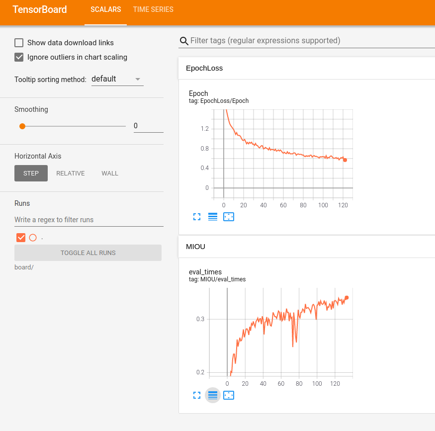
tensorboard
使用很简单的,看下面代码就懂了
1
2
3
4
5
6
7
8
9
10
11
12
13
14
from torch.utils.tensorboard import SummaryWriterimport ostest= SummaryWriter('run' ) for i in range (10 ): test.add_scalar('Train/loss' , i * 100 + 1 , i) test.add_scalar("test" , i * 200 + 1 , i) test.close() os.system("tensorboard --logdir=run" )
如果是使用ssh连接服务器如何查看tensorboard的图像呢?
连接ssh时,将服务器的6006端口重定到自己的机器上来
1 ssh -L 16006:127.0.0.1:6006 username@ip
其中:16006:127.0.0.1:6006表示自己机器上的16006号端口,6006是服务器上的tensorboard使用的端口
在服务上使用6006端口正常启动tensorboard
1 tensorboard --logdir==xxx --port=6006
在本地浏览器中输入下面的网页地址即可查看tensorboard
设置固定用哪张卡
torch.cuda.set_device(card_id),card_id是卡的编号
使用这个方法似乎只能针对在某张卡上训练,但是加载模型的时候还是会使用默认卡(暂时不确定是版本问题还是操作系统的问题)
因此在设置好torch.cuda.set_device(card_id)后,在torch.load()时,加入参数map_loaction="cuda:card_id"card_id还是之前卡的编号,这样就能把模型加载到指定的卡上了,当然如果想使用torch.cuda.is_available()确定可以使用在载入显卡时可以使用model.cuda(card_id)这样实现在对应卡中加载模型
在训练中进行验证爆显存问题
使用with torch.no_grad()就可以解决了
1
2
with torch.no_grad(): 验证代码
使用字典参数的形式对模型进行修改
核心思想是在模型文件中进行修改,在加载参数时将预训练模型的参数存到字典里,并从其中提取新模型层需要的参数,然后重新加载,保存模型
1
2
3
4
5
6
7
8
9
10
11
12
13
14
15
16
17
18
19
20
21
22
23
import torchfrom models.model_stages import BiSeNetmodel = BiSeNet(backbone="STDCNet1446" , n_classes=19 , pretrain_model=None , use_boundary_2=False , use_boundary_4=False , use_boundary_8=True , use_boundary_16=False , use_conv_last=False ) model.eval () originParams = torch.load("./checkpoints/STDC2-Seg/model_maxmIOU75.pth" ) modelDict = model.state_dict() pullDict = {name: value for name, value in originParams.items() if name in modelDict.keys()} modelDict.update(pullDict) model.load_state_dict(modelDict) torch.save(model, "STDC2.pth" ) print ("save finished!" )
万恶的NinJa
问题描述:RuntimeError: Ninja is required to load C++ extension
1
2
3
wget https://github.com/ninja-build/ninja/releases/download/v1.8.2/ninja-linux.zip sudo unzip ninja-linux.zip -d /usr/local/bin/ sudo update-alternatives --install /usr/bin/ninja ninja /usr/local/bin/ninja 1 --force
特征图可视化
先说说特征图可视化到底在可视什么,我们都知道一次卷积计算最后只会产生一张特征图,也就是通道为1的图,但是通常我们的卷积都不止一个通道,实际上是因为卷积核的数量不止一个,所以就可以出现多张特征图叠加的情况。
所以特征图可视化不可能把所有的卷积核出来的结果都显示出来,所以会选择几层进行展示,直接上代码吧
1 2 3 4 5 6 7 8 9 10 11 12 13 14 15 16 def visual (module, inputs, outputs ): x = inputs[0 ][0 ] y = outputs[0 ] for i in range (10 ): plt.imshow(x[i].detach().cpu().numpy()) plt.savefig(f"visiable/featuremap/input{i} .jpg" ) plt.imshow(y[i].detach().cpu().numpy()) plt.savefig(f"visiable/featuremap/output{i} .jpg" ) net = torch.load(model_path, map_location='cpu' ) for name, m in net.named_modules(): if isinstance (m, 这里填填要查看模块的类名): m.register_forward_hook(visual)
cv2无法使用imwrite和imread读取中文路径的图片咋办
1 2 3 4 img = cv2.imdecode(np.fromfile(self .path, dtype=np.uint8), -1 ) cv2.imencode('.png' , img)[1 ].tofile(self .mask_total_path)
Picgo+Gitee配置图床
打开偏好设置,选择PicGo-Core(command line),然后打开配置文件,然后会打开config.json,文件将下面这个内容复制过去修改一下就行了
1
2
3
4
5
6
7
8
9
10
11
12
13
14
15
16
17
18
19
20
21
{ "picBed" : { "uploader" : "gitee" , "current" : "gitee" , "gitee" : { "repo" : "用户名/仓库名" , "branch" : "分支" , "token" : "Token" , "path" : "" , "customPath" : "default" , "customUrl" : "" } , "transformer" : "path" } , "picgoPlugins" : { "picgo-plugin-gitee-uploader" : true } , "picgo-plugin-gitee-uploader" : { "lastSync" : "2021-11-14 11:05:49" } }
指标类
miou
1 2 3 4 5 6 7 8 9 10 11 12 13 14 15 def fast_hist (res, gt, classes ): k = (res >= 0 ) & (res < classes) return torch.bincount(classes * res[k] + gt[k], minlength=classes**2 ).reshape(classes, classes) def iou_per_class (hist ): return hist.diag() / (hist.sum (dim=0 ) + hist.sum (dim=1 ) - hist.diag())
mae
1
2
3
def mae (res, gt ): return torch.mean(torch.abs (res - gt))
F β F_{\beta} F β 1 2 3 4 def fb (hist, beta2=0.3 ): precision = hist[1 , 1 ] / (hist[1 , 1 ] + hist[0 , 1 ]) recall = hist[1 , 1 ] / (hist[1 , 1 ] + hist[1 , 0 ]) return (1 + beta2) * precision * recall / (beta2 * precision + recall)
NMI(归一化互信息)
互信息可以衡量两个分布之间的依赖程度,判断两种分布的一致性。
假设对10个样本点进行聚类,运用聚类算法得到的结果为:
A = [1,1,1,2,2,3,2,1,3,3]
标准聚类结果为:
B = [1,1,2,3,2,1,1,1,3,2]
令X = unique(A)=[1,2,3],Y = unique(B)=[1,2,3]
互信息(MI)的计算公式为:
M ( X , Y ) = ∑ i = 1 ∣ X ∣ ∑ j = 1 ∣ Y ∣ P ( i , j ) log ( P ( i , j ) P ( i ) P ‘ ( j ) ) \boldsymbol{M}(X, Y)=\sum_{i=1}^{|X|} \sum_{j=1}^{|Y|} \boldsymbol{P}(i, j) \log \left(\frac{\boldsymbol{P}(i, j)}{\boldsymbol{P}(i) P^{`}(j)}\right)
M ( X , Y ) = i = 1 ∑ ∣ X ∣ j = 1 ∑ ∣ Y ∣ P ( i , j ) log ( P ( i ) P ‘ ( j ) P ( i , j ) )
其中P ( i , j ) \boldsymbol{P}(i,j) P ( i , j ) P ( i , j ) = ∣ X i ∩ Y j ∣ N P(i, j)=\frac{\left|X_{i} \cap Y_{j}\right|}{N} P ( i , j ) = N ∣ X i ∩ Y j ∣
按照上面的例子
P ( 1 , 1 ) = 3 10 , P ( 1 , 2 ) = 1 10 , P ( 1 , 3 ) = 0 , P(1,1)=\frac 3{10},P(1,2)=\frac 1{10},P(1,3)=0, P ( 1 , 1 ) = 10 3 , P ( 1 , 2 ) = 10 1 , P ( 1 , 3 ) = 0 ,
P ( 2 , 1 ) = 1 10 , P ( 2 , 2 ) = 1 10 , P ( 2 , 3 ) = 1 10 , P(2,1)=\frac 1{10},P(2,2)=\frac 1{10},P(2,3)=\frac 1{10}, P ( 2 , 1 ) = 10 1 , P ( 2 , 2 ) = 10 1 , P ( 2 , 3 ) = 10 1 ,
P ( 3 , 1 ) = 1 10 , P ( 3 , 2 ) = 1 10 , P ( 3 , 3 ) = 1 10 P(3,1)=\frac 1{10},P(3,2)=\frac 1{10},P(3,3)=\frac 1{10} P ( 3 , 1 ) = 10 1 , P ( 3 , 2 ) = 10 1 , P ( 3 , 3 ) = 10 1
然后计算分母中的概率函数P ( i ) = X i N P(i) = \frac {X_i}N P ( i ) = N X i P ‘ ( j ) = Y i N P^`(j) = \frac {Y_i}N P ‘ ( j ) = N Y i
按照上面的例子
P ( 1 ) = 4 10 , P ( 2 ) = 3 10 , P ( 3 ) = 3 10 P(1)=\frac 4{10},P(2)=\frac 3{10},P(3)=\frac 3{10} P ( 1 ) = 10 4 , P ( 2 ) = 10 3 , P ( 3 ) = 10 3
P ‘ ( 1 ) = 5 10 , P ‘ ( 2 ) = 3 10 , P ‘ ( 3 ) = 2 10 P^`(1)=\frac 5{10},P^`(2)=\frac 3{10},P^`(3)=\frac 2{10} P ‘ ( 1 ) = 10 5 , P ‘ ( 2 ) = 10 3 , P ‘ ( 3 ) = 10 2
这样就可以算出互信息了
标准化互信息的公式如下:
N M I ( X , Y ) = 2 M I ( X , Y ) H ( X ) + H ( Y ) NMI(X,Y) = \frac{2MI(X,Y)}{H(X)+H(Y)}
NM I ( X , Y ) = H ( X ) + H ( Y ) 2 M I ( X , Y )
H ( X ) , H ( Y ) H(X),H(Y) H ( X ) , H ( Y )
H ( X ) = − ∑ i = 1 ∣ X ∣ P ( i ) l o g ( P ( i ) ) H ( X ) = − ∑ j = 1 ∣ X ∣ P ‘ ( j ) l o g ( P ‘ ( j ) ) H(X) = -\sum_{i=1}^{|X|}P(i)log(P(i))\\
H(X) = -\sum_{j=1}^{|X|}P^`(j)log(P^`(j))\\
H ( X ) = − i = 1 ∑ ∣ X ∣ P ( i ) l o g ( P ( i )) H ( X ) = − j = 1 ∑ ∣ X ∣ P ‘ ( j ) l o g ( P ‘ ( j ))
这样就是标准化互信息的计算方式了
实现代码很简单
1 2 3 4 from sklearn import metricsA = np.array([1 ,1 ,1 ,2 ,2 ,3 ,2 ,1 ,3 ,3 ]) B = np.array([1 ,1 ,2 ,3 ,2 ,1 ,1 ,1 ,3 ,2 ]) print (metrics.normalized_mutual_info_score(A,B))
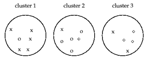
PUR(纯度,Purity)
这个和accuracy相似,是聚类的常见指标。计算公式为P u r i t y = ∑ i = 1 k m i m p i Purity=\sum_{i=1}^k\frac{m_i}mp_i P u r i t y = ∑ i = 1 k m m i p i
举个例子:
假设有17个样本有3个聚类,在第一个中,x比较多应该是属于x的聚类,正确聚类的有5个;在第二个中○比较多应该是属于○的,正确聚类有4个;在第三个中◇比较多,应该是属于◇的,正确聚类的有3个。于是纯度的计算方式为5 + 4 + 3 17 = 0.7059 \frac {5+4+3}{17}=0.7059 17 5 + 4 + 3 = 0.7059
代码实现:
1 2 3 4 5 6 7 8 9 10 11 12 13 14 15 16 17 18 19 20 21 22 23 24 25 26 27 28 29 30 31 32 33 34 35 36 37 38 39 40 41 42 from sklearn.metrics import accuracy_scoreimport numpy as npdef purity_score (y_true, y_pred ): """Purity score Args: y_true(np.ndarray): n*1 matrix Ground truth labels y_pred(np.ndarray): n*1 matrix Predicted clusters Returns: float: Purity score """ y_voted_labels = np.zeros(y_true.shape) labels = np.unique(y_true) ordered_labels = np.arange(labels.shape[0 ]) for k in range (labels.shape[0 ]): y_true[y_true==labels[k]] = ordered_labels[k] labels = np.unique(y_true) bins = np.concatenate((labels, [np.max (labels)+1 ]), axis=0 ) for cluster in np.unique(y_pred): hist, _ = np.histogram(y_true[y_pred==cluster], bins=bins) winner = np.argmax(hist) y_voted_labels[y_pred==cluster] = winner return accuracy_score(y_true, y_voted_labels) y_true = np.array([0 , 0 , 0 , 1 , 1 , 1 , 2 ]) y_pre = np.array([1 , 1 , 1 , 2 , 2 , 2 , 2 ]) print (purity_score(y_true,y_pre))
参数量与计量获取
1
2
3
4
5
6
7
8
9
from thop import profilenet.eval () a = torch.rand((1 , 3 , 320 , 320 )) flops, params = profile(net, inputs=(a,)) print (flops)print (params)print ('FLOPs = ' + str (flops / 1000 ** 3 ) + 'G' )print ('Params = ' + str (params / 1000 ** 2 ) + 'M' )exit(0 )
服务器开启jupyter lab
先安装
生成配置文件
1 jupyter lab --generate-config
修改对应的配置文件vi ~/.jupyter/jupyter_lab_config.py 为如下内容
1
2
3
4
5
6
7
c.ServerApp.ip = '*' c.ServerApp.port = 9999 # jupyter lab要使用的端口 c.ServerApp.open_browser = False c.ServerApp.root_dir = 'path' # jupyter lab启动后进入的根路径,对根路径下的所有文件都有访问权限 c.ServerApp.password_required = True # 是否需要密码 c.ServerApp.password = 'password' # 这两个好像都是密码,设置成一样的就行 c.NotebookApp.token = 'password'
启动指令
使用ip address查看一下公网或内网ip地址,然后本机访问https:\\服务器ip:jupyter lab端口即可,比如,假设服务器IP为45.16.233.154,则按照上面的配置方式访问的地址就是https:\\45.16.233.154:9999