「论文阅读」Dual Contrastive Prediction for Incomplete Multi-View Representation Learning

论文名称：Dual Contrastive Prediction for Incomplete Multi-View Representation Learning

作者：Yijie Lin; Yuanbiao Gou; Xiaotian Liu; Jinfeng Bai; Jiancheng Lv; Xi Peng

期刊：IEEE Transactions on Pattern Analysis and Machine Intelligence

时间：2022-8

原文摘要

In this article, we propose a unifified framework to solve the following two challenging problems in incomplete multi-view representation learning: i) how to learn a consistent representation unifying different views, and ii) how to recover the missing views. To address the challenges, we provide an information theoretical framework under which the consistency learning and data recovery are treated as a whole. With the theoretical framework, we propose a novel objective function which jointly solves the aforementioned two problems and achieves a provable suffificient and minimal representation. In detail, the consistency learning is performed by maximizing the mutual information of different views through contrastive learning, and the missing views are recovered by minimizing the conditional entropy through dual prediction. To the best of our knowledge, this is one of the fifirst works to theoretically unify the cross-view consistency learning and data recovery for representation learning. Extensive experimental results show that the proposed method remarkably outperforms 20 competitive multi-view learning methods on six datasets in terms of clustering, classifification, and human action recognition. The code could be accessed from https://pengxi.me.

理论基础

多视图表征学习(MVRL)的目的是学习一个函数$f$，映射多视图数据到低维的空间中，这个低维空间中学习到的公共表示将被用于下游任务，比如聚类，分类以及人类行为识别等。为了达到这个目标，关键是从不同的视图中学习到一致性信息。

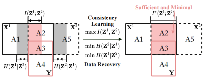
在上图$\mathbf{X}^1$和$\mathbf{X}^2$表示给定数据集的两个视图，$\mathbf{Z}^1$和$\mathbf{Z}^2$分别对应相应的representation，$\mathbf{X}^1=\mathrm{A} 1 \cup \mathrm{A} 2 \cup \mathrm{A} 3$和$\mathbf{X}^2=\mathrm{A} 2 \cup \mathrm{A} 3 \cup \mathrm{A} 3$ 包含的信息分别对应实线和虚线矩形，下方的红色矩形框$(\mathbf{Y}=\mathrm{A} 3 \cup \mathrm{A} 4)$表示任务相关的信息。具体来说，$A1(\left(H\left(\mathbf{X}^1 \mid \mathbf{X}^2\right)\right))$和$A5\left(H\left(\mathbf{X}^2 \mid \mathbf{X}^1\right)\right)$表示$\mathbf{X}^1$和$\mathbf{X}^2$的视图特定信息。 $\mathrm{A} 2\left(I\left(\mathbf{X}^1 ; \mathbf{X}^2 \mid \mathbf{Y}\right)\right)$和$\mathrm{A} 3\left(I\left(\mathbf{X}^1 ; \mathbf{X}^2 ; \mathbf{Y}\right)\right)$一起表示$\mathbf{X}^1$和$\mathbf{X}^2$的互信息，其中$A3$是任务相关的信息，而$A2$是任务无关的信息。$A4\left(H\left(\mathbf{Y} \mid \mathbf{X}^1, \mathbf{X}^2\right)\right)$表示无法从输入数据中得到的任务相关信息。

本文分别使用互信息(红色的面积)$I\left(\mathbf{Z}^1 ; \mathbf{Z}^2\right)$和条件熵(灰色的面积)$H\left(\mathbf{Z}^i \mid \mathbf{Z}^j\right.)$量化跨视图一致性和跨视图恢复性，最大化互信息$I\left(\mathbf{Z}^1 ; \mathbf{Z}^2\right)$同时最小化条件熵$H\left(\mathbf{Z}^i \mid \mathbf{Z}^j\right)$。于是两个目标能够相互增强并联合优化以得到足够($\mathrm{A} 3 \in \mathbf{Z}^i$)且最小($(\mathrm{A} 1 \cup \mathrm{A} 5) \notin \mathbf{Z}^i$ and $A2 \in \mathbf{Z}^i$)的representation。

充分的representation指为下游任务学习了足够的信息

最小的representation指所有与任务无关的信息都以一个固定的间隙被删除

任务与存在的问题

不完整视图问题(IMP)需要解决两个问题

1. 如何从不同的视图中学习一致性表征
2. 如何在不完整的数据中恢复缺失的视图

主要工作和创新点

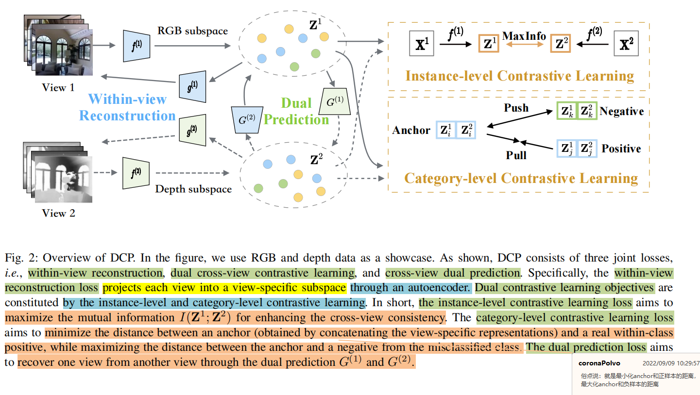
本文提出了一个不完整多视图表征学习方法，称为双对比预测(Dual Contrastive Prediction, DCP)。DCP映射高维数据到一个潜在空间中，这个空间的跨视图一致性和数据恢复性收到三个联合损失的监督

1. 视图内重构损失：学习视图特定的representation同时保留原始信息
2. 双对比损失：通过最大化互信息$I\left(\mathbf{Z}^1 ; \mathbf{Z}^2\right)$学习跨视图一致性
3. 双预测损失：通过最小化条件熵$H\left(\mathbf{Z}^1 \mid \mathbf{Z}^2\right.)$和$H\left(\mathbf{Z}^2 \mid \mathbf{Z}^1\right.)$恢复缺失的视图。

主要贡献：

1. 在信息论的框架下，交叉视图一致性学习和数据恢复的内在联系。
2. 提出DCP通过双对比损失和双预测损失分别得到信息一致性和数据恢复性
3. 为了利用可用的标签信息，DCP设计并利用了实例级别和类级别的对比损失以增强representation的可分性。

提出的方法

$\mathbf{X}^1$和$\mathbf{X}^2$表示相同实例的不同视图，其标签为$\mathbf{Y}$。$\mathbf{Z}^i$为视图$\mathbf{X}^i$的representation，其通过一个确定的映射$f^{(i)}:\mathbf{Z}^i(\mathbf{X}^i)$获得，$i=1,2$。使用$H(A)$表示熵，$H(A|B)$表示条件熵，$I(A;B)$表示互信息，$I(A;B|C)$表示条件互信息。

定义1：跨视图一致性

给定视图特定的representation $\mathbf{Z}^i$和$\mathbf{Z}^j$，对于任意的$\mathbf{Z}^{\prime}\in\tau(\mathbf{X}^j)$和$\mathbf{Z}^{\prime\prime}\in\tau(\mathbf{X}^i)$，其中$\tau(\mathbf{X}^v)$是第v个视图$\mathbf{X}^v$的possible latent representation的集合，如果$I(\mathbf{Z}^i,\mathbf{Z}^j)\geq I(\mathbf{Z}^i;\mathbf{Z}^{\prime})$并且$I(\mathbf{Z}^i,\mathbf{Z}^j)\geq I(\mathbf{Z}^{\prime\prime};\mathbf{Z}^j)$，那么$\mathbf{Z}^i$和$\mathbf{Z}^j$是一致的。

定义2：跨视图可恢复性

给定representation $\mathbf{Z}^i$，对于任意的$\mathbf{Z}^{\prime}\in\tau(\mathbf{X}^j)$，如果$H(\mathbf{Z}^i|\mathbf{Z}^j)\leq H(\mathbf{Z}^i|\mathbf{Z}^{\prime})$，那么$\mathbf{Z}^i$是可恢复的。当且仅当$H(\mathbf{Z}^i|\mathbf{Z}^j)=0$时$\mathbf{Z}^i$是完全可恢复的。

定义2中的恢复指的是恢复视图的公共信息，而不是全部信息，恢复公共信息有助于提高框架在下游任务中的表现。

理论1：一致性和可恢复性的等价性

若representation $\mathbf{Z}^i$和$\mathbf{Z}^j$跨视图一致，当且仅当$\mathbf{Z}^i$对于$\mathbf{Z}^j$是可恢复的并且$\mathbf{Z}^j$对于$\mathbf{Z}^i$也是可恢复的(证明略)

假设1：多视图数据的同等充分性

对于下游任务，每一个视图的sufficency是近似相等的，比如保持$I\left(\mathbf{X}^1 ; \mathbf{Y}\right)=I\left(\mathbf{X}^2 ; \mathbf{Y}\right)=I\left(\mathbf{X}^1 ; \mathbf{X}^2 ; \mathbf{Y}\right)$

观点1：$I\left(\mathbf{X}^1 ; \mathbf{Y} \mid \mathbf{X}^2\right)=I\left(\mathbf{X}^2 ; \mathbf{Y} \mid \mathbf{X}^1\right)=0$(证明略）

定义3：Sufficient Representation

对于representation $\mathbf{Z}^1$和$\mathbf{Z}^2$，如果$I\left(\mathbf{Z}^1 ; \mathbf{Y}\right)=I\left(\mathbf{Z}^2 ; \mathbf{Y}\right)=I\left(\mathbf{X}^1 ; \mathbf{X}^2 ; \mathbf{Y}\right)$，那么$\mathbf{Z}^1$和$\mathbf{Z}^2$是sufficent的。sufficient representation监督从输入中得到的足够的用于下游任务的信息。

定义4：Minimal Representation

对于representation $\mathbf{Z}^1$和$\mathbf{Z}^2$，如果$I\left(\mathbf{Z}^1 ; \mathbf{X}^1 \mid \mathbf{Y}\right)=I\left(\mathbf{Z}^2 ; \mathbf{X}^2 \mid \mathbf{Y}\right)=I\left(\mathbf{X}^1 ; \mathbf{X}^2 \mid \mathbf{Y}\right)$，那么$\mathbf{Z}^1$和$\mathbf{Z}^2$是minimal的。minimal representation期望能够去除任务无关的信息，保留固定的间隙$I\left(\mathbf{X}^1 ; \mathbf{X}^2 \mid \mathbf{Y}\right)$

损失函数

sufficient和minimal的MVRL的通用形式为：

$$公式1： \begin{align} & \max I\left(\mathbf{Z}^1 ; \mathbf{Z}^2\right)\\ & s.t. \min H\left(\mathbf{Z}^1 \mid \mathbf{Z}^2\right), \min H\left(\mathbf{Z}^2 \mid \mathbf{Z}^1\right) \end{align}$$

上图是DCP的结构图，其由3个联合学习目标组成，视图内重构损失$\mathcal{L}_{rec}$，跨视图双流对比损失$\mathcal{L}_{cl}$，跨视图双流预测损失$\mathcal{L}_{pre}$，最终的损失函数可以表示为：

$$公式2：\mathcal{L}=\mathcal{L}_{cl}+\lambda_1\mathcal{L}_{pre}+\lambda_2\mathcal{L}_{rec}$$

其中$\lambda_1$和$\lambda_2$平衡了$\mathcal{L}_{pre}$和$\mathcal{L}_{rec}$。在实验中，这两个平衡因子都设置为0.1。

视图内重构损失

对于给定的数据集$\overline{\mathbf{X}}=\left\{\overline{\mathbf{X}}^{(1,2)}, \overline{\mathbf{X}}^{(1)}, \overline{\mathbf{X}}^{(2)}\right\}$，其由n个样本，$\overline{\mathbf{X}}^{(1,2)}, \overline{\mathbf{X}}^{(1)}$, 和$\overline{\mathbf{X}}^{(2)}$ 分别表示在每个视图中共同显示的部分，只在第一个视图显示的部分，只在第二个视图显示的部分。具体来说$\overline{\mathbf{X}}^{(1,2)}$表示包含m个样本的完整数据集，而$\mathbf{X}^v$表示第v个视图的数据，其中可能包含不完整的数据的样本。

第v个视图的数据通过一个特定的编码器得到representation $\mathbf{Z}^v$，其使用$\mathcal{L}_{rec}$进行优化，具体公式如下：

$$公式3：\mathcal{L}_{r e c}=\sum_{v=1}^2 \sum_{t=1}^m\left\|\mathbf{X}_t^v-g^{(v)}\left(\mathbf{Z}_t^v\right)\right\|_2^2$$

其中$\mathbf{X}_t^v$表示$\mathbf{X}^v$的第t个样本，$g^{(v)}$是第v个视图的解码器，representation $\mathbf{Z}_t^v$的定义如下：

$$公式4：\mathbf{Z}_t^v=f^{(v)}\left(\mathbf{X}_t^v\right),$$

其中$f^{(v)}$是第v个视图的编码器。

双对比学习损失

使用对比学习来最大化多视图的一致性，以克服在不完整视图表征学习中的一致性学习挑战。其由实例级和类级约束损失构成，可以用下面的公式表示

$$公式5：\mathcal{L}_{c l}=\mathcal{L}_{i c l}+\mathcal{L}_{c c l},$$

其中实例级对比损失 $\mathcal{L}_{i c l}$尝试学习有信息和一致性的representation，在没有标签的帮助下用于不同的视图。类级对比损失 $\mathcal{L}_{c c l}$的目的是使用标签信息来增强可分性。

实例级对比学习：在使用自编码器学习的潜在特征空间中，使用对比学习最大化跨不同视图的一致性。本文提出直接最大化不同视图的representation之间的互信息。可以用下面的公式表示：

$$公式6：\mathcal{L}_{i c l}=-\sum_{t=1}^m\left(I\left(\mathbf{Z}_t^1 ; \mathbf{Z}_t^2\right)+\alpha\left(H\left(\mathbf{Z}_t^1\right)+H\left(\mathbf{Z}_t^2\right)\right)\right),$$

其中$I$和$H$分别表示互信息和熵，平衡因子$\alpha=9$用于正则化熵。

$\left\{\mathbf{Z}^i\right\}_{i=1}^2$可以被认为是两个离散聚类分布变量$z$和$z^{\prime}$在D类上的分布，其中D表示的是维数。理论上，我们能够使用$\mathbf{P} \in \mathcal{R}^{D \times D}$定义联合概率分布$\mathcal{P}\left(z, z^{\prime}\right)$如下：

$$公式7：\mathbf{P}=\frac{1}{m} \sum_{t=1}^m \mathbf{Z}_t^1\left(\mathbf{Z}_t^2\right)^{\top}$$

边缘概率分布$\mathcal{P}(z=d)$和$\mathcal{P}\left(z^{\prime}=d^{\prime}\right)$分别表示为$\mathbf{P}_d$和$\mathbf{P}_d^{\prime}$。他们能够通过对联合概率分布$\mathbf{P}$的第$d$行和第$d^{\prime}$列求和得到。因此，公式6可以写为

$$公式8：\mathcal{L}_{i c l}=-\sum_{d=1}^D \sum_{d^{\prime}=1}^D \mathbf{P}_{d d^{\prime}} \ln \frac{\mathbf{P}_{d d^{\prime}}}{\mathbf{P}_d^{\alpha+1} \cdot \mathbf{P}_{d^{\prime}}^{\alpha+1}},$$

其中$\mathbf{P}_{d d^{\prime}}$是$\mathbf{P}$的第$d$行和第$d^{\prime}$列，$\alpha$和公式6中定义的平衡因子相同。

类级对比学习：利用可用的标签信息去引导representation学习，在无监督学习中则不使用类级对比损失函数$\mathcal{L}_{ccl}$。在$\mathbf{Z}_t=\left[\mathbf{Z}_t^1 ; \mathbf{Z}_t^2\right]$上执行$\mathcal{L}_{ccl}$，其中$[;]$表示拼接操作

$$公式9：\mathcal{L}_{c c l}=\sum_t^m\left[\mathbb{E}_{\mathbf{Z} \sim \mathcal{T}(y)} S\left(\mathbf{Z}, \mathbf{Z}_t\right)-\mathbb{E}_{\mathbf{Z} \sim \mathcal{T}(g t)} S\left(\mathbf{Z}, \mathbf{Z}_t\right)+\gamma\right]_{+}$$

其中$g t$是$\mathbf{Z}_t, S\left(\mathbf{Z}, \mathbf{Z}_t\right)=\mathbf{Z}^T \mathbf{Z}_t$的ground truth，$\mathbf{Z}_t, S\left(\mathbf{Z}, \mathbf{Z}_t\right)=\mathbf{Z}^T \mathbf{Z}_t$是点积形式的相似度函数。$\mathcal{T}(g t)$是从ground truth标签$gt$得到的公共representation集合。$\mathcal{T}(y)$是从预测$y$中得到的representation集合。$\gamma$是一个非负的常数，当预测正确时$\gamma=0$，预测错误时$\gamma=1$，预测标签$y$可以用下面的方法计算：

$$公式10：y=\underset{y \in \mathcal{Y}}{\arg \max } \mathbb{E}_{\mathbf{Z} \sim \mathcal{T}(y)} S\left(\mathbf{Z}, \mathbf{Z}_t\right) .$$

双预测损失

使用一个变分分布$\mathcal{Q}\left(\mathbf{Z}^i \mid \mathbf{Z}^j\right)$并最大化其下界$\mathbb{E}_{\mathcal{P}_{\mathbf{Z}^i, \mathbf{Z}^j}}\left[\log \mathcal{P}\left(\mathbf{Z}^i \mid \mathbf{Z}^j\right)\right]$近似计算条件熵$H\left(\mathbf{Z}^i \mid \mathbf{Z}^j\right)$。这个变分分布$\mathcal{Q}$可以当做是一个高斯分布$\mathcal{N}\left(\mathbf{Z}^i \mid G^{(j)}\left(\mathbf{Z}^j\right), \sigma \mathbf{I}\right)$，其中$\sigma \mathbf{I}$是方差矩阵，$G^{(j)}(\cdot)$是从$\mathbf{Z}^j$中回复$\mathbf{Z}^i$的参数模型。期望的最大化$\mathbb{E}_{\mathcal{P}_{\mathbf{Z}^i, \mathbf{Z}^j}}\left[\log \mathcal{Q}\left(\mathbf{Z}^i \mid \mathbf{Z}^j\right)\right]$等价于

$$公式11：\min \mathbb{E}_{\mathcal{P}_{\mathbf{Z}^i, \mathbf{Z}^j}}\left\|G^{(j)}\left(\mathbf{Z}^j\right)-\mathbf{Z}^i\right\|_2^2$$

考虑两个视图数据，双预测损失可以用下面的形式表示：

$$公式12：\mathcal{L}_{\text {pre }}=\left\|G^{(1)}\left(\mathbf{Z}^1\right)-\mathbf{Z}^2\right\|_2^2+\left\|G^{(2)}\left(\mathbf{Z}^2\right)-\mathbf{Z}^1\right\|_2^2$$

在训练完成后，使用整个数据集到网络中，并得到所有视图的representation，对于缺失视图（$\overline{\mathbf{X}}^{(1)}, \overline{\mathbf{X}}^{(2)}$），我们通过双流预测，从已有的representation $\overline{\mathbf{Z}}^{(j)}$中恢复缺失的表征$\hat{\mathbf{Z}}^{(i)}$

$$公式13：\hat{\mathbf{Z}}^{(i)}=G^{(j)}\left(\overline{\mathbf{Z}}^{(j)}\right)=G^{(j)}\left(f^{(j)}\left(\overline{\mathbf{X}}^{(j)}\right)\right)$$

其中$\overline{\mathbf{Z}}^{(j)}$是$\overline{\mathbf{X}}^{(j)}$的representation。通过简单地拼接所有的视图特定representation来推导出公共representation $\mathbf{Z}$。具体来说，对于完整的样本，$\mathbf{Z}=\left[\mathbf{Z}^1 ; \mathbf{Z}^2\right]$，对于不完整的样本，$\mathbf{Z}=\left[\hat{\mathbf{Z}}^{(1)} ; \overline{\mathbf{Z}}^{(2)}\right]$，或者$\mathbf{Z}=\left[\overline{\mathbf{Z}}^{(1)} ; \hat{\mathbf{Z}}^{(2)}\right]$

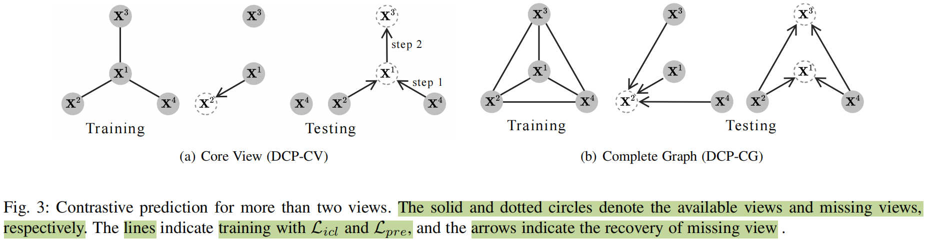
用于多个视图的对比预测

有两种通用的公式去解决多个视图的对比预测问题：基于核心视图的方法(DCP-CV)，基于完整图的方法(DCP-CG)

给定有$V$个视图的数据集$\left\{\mathbf{X}^i\right\}_{i=1}^V$，DCP-CV选择一个重要的视图作为中心，按照下面的公式执行$\mathbf{X}^1$和其他视图$\mathbf{X}^j$之间的双对比预测：

$$公式14：\mathcal{L}_{\mathrm{DCP}-\mathrm{CV}}=\sum_{i=2}^V \mathcal{L}_{i p}\left(\mathbf{Z}^1, \mathbf{Z}^i\right)+\lambda_2 \sum_{i=1}^V \mathcal{L}_{\text {rec }}\left(\mathbf{Z}^i\right)+\mathcal{L}_{c d}$$

其中$\mathcal{L}_{i p}=\mathcal{L}_{i c l}+\lambda_1 \mathcal{L}_{p r e}, \lambda_1$，$\lambda_1$和$\lambda_2$和公式2中的定义相同，使用公共representation实现类级对比损失$\mathcal{L}_{\text {ccl }}$

DCP-CG在所有可能的视图对上执行实例级对比学习和双约束，

$$公式15：\mathcal{L}_{\mathrm{DCP-CG}}=\sum_{1 \leq i<j \leq V} \mathcal{L}_{i p}\left(\mathbf{Z}^i, \mathbf{Z}^j\right)+\lambda_2 \sum_{i=1}^V \mathcal{L}_{r e c}\left(\mathbf{Z}^i\right)+\mathcal{L}_{c c l}$$

虽然DCP-CV和DCP-CG都能够学习足够和最小的representation，但我们推荐后者的原因如下：一方面，为了一致性学习，DCP-CG将捕获更多的信息，因为所有的视图对都在学习阶段被包含和利用。DCP-CG视图最大化$v(v-1)/2$次，而DCP-CV值最大化$v-1$次。另一方面，DCP-CG比DCP-CV再执行数据恢复方面展示出更强的鲁棒性。